Optimizing Disk IO Through Abstraction

To Engineer or Not To…

When disk capacity is released to a new application or service many times the projects do not consider how best to use the storage that has been provided. Essentially the approaches fall into one of two schools of thought. The first is to reduce upfront engineering into a couple design options and resolve issues when they arise. The second is to engineer several solution sets with variable parameters that will provide a broader pallet of solutions and policies from which an appropriate solution may be selected.

Reduced Simplified Engineering

• Apply one of a couple infrastructure designs to a project.
• This approach involves less work upfront, has a simpler execution and involves less work gathering requirements.
• Potentially more time and effort will be spent resolving issues when resources and design are insufficient.

Solution Engineering

• Develop several standard solution sets and models and document policies and procedures which will be used to fit applications/components into these models.
• This approach involves substantial requirements gathering and entails more work and complexity.
• The result is a more efficient use of resources and less time spent resolving issues because the design and resources should better fit the system needs.

Engineering Disk Performance

When it comes to disk performance the cost of not considering how to optimize the use of the storage infrastructure can be very significant. Consider the IO operation cycle time table. The order of magnitude difference between CPU operations, memory operations and that of device IO is significant. If cycle time is scaled up to a second the comparative difference is between seconds and that of device IO taking months to years to complete. Poorly orchestrated device use cases can result in significant impact. A memory miss will only cost a few hundred nanoseconds but a disk IO cycle miss could cost a couple dozen milliseconds. To put it in the perspective of scale we are talking about the difference between four minutes and eight months.

Device	Cycle Time	Cycle in Seconds	Scaled Cycle
CPU	1 nanosecond	1.00×10^-9	1	seconds
CPU Register	5 nanoseconds	5.00×10^-9	5	seconds
Memory	100 nanoseconds	1.00×10^-7	2	minutes
Disk	10 milliseconds	1.00×10^-2	4	months
NFS Op	50 milliseconds	5.00×10^-2	2	years
Tape	10 seconds	1.00×10^1	3	centuries

IO Op Cycle Time Scales

How IO devices are use by systems can impact device performance in several ways. First, between the system and the device is usually a cache which attempts to predict what data will be needed and pre-stages it in faster memory in anticipation of any potential access requests. Traditional cache algorithms identify data that is accessed in ordered proximity on the IO device and then reads ahead to pre-fetch subsequent data. These pages are then left in cache until they are aged out due to subsequent access to other data on the device. The result is that sequential IOs will experience better performance because the data will be in cache. However random IOs and IOs that occur sporadically will require direct access to the slower storage device. Newer caching algorithms such as SARC have algorithms designed to improve anticipation of random IO but are no substitute for considering data layout on the devices. An example of incorrect data layout would be over aggressive server side striping using volume management which can cause sequential IOs on the system to appear as random on the storage device; in essence, circumventing caching. The second area of consideration is the storage device back-end performance. Back-end performance can be impacted by IO sizes and distributions across array boundaries. The most significant impact comes from conflicting IOs that request data from different portions of storage device media at the same time. The result is what is termed “thrashing” because the device access mechanism must be readdressed from one part of the media to another requiring increased times for continuous repositioning.

Optimizing the Layout of Information on Storage

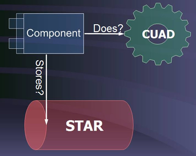
With all these potential factors that can impact storage performance how can a method for optimizing how storage devices are used be formulated? Some of the decisions have to be made on the back-end by the Storage Analysts that configure and present the storage to hosts. Once storage is presented to a host how the storage is used in light of these factors needs to be considered. Back-end configuration considerations vary by storage device implementation but most storage sub-systems have facilities that automate redistribution of data to balance IOs across the device media. Directions on optimum logical device configuration on the storage system are available in architecture documentation and from field engineers. But once these configured devices are made available to a system a method of laying out data needs to be considered that will increase sequential IO and reduce IO conflict potential. To develop a standard method rather then create unique custom solutions for each application component is more advantageous to establish a more predictable, re-creatable and supportable environment. This method should consider three factors. It should consider what the component does, what the component stores and how large of an implementation the component is supporting.

Categorizing Component Functionality

The first step is to determine what an application component does. Some applications are a single entity while other applications are non-monolithic and break the work they perform down into subsets of functionality performed by components. All applications or component functionality can be categorized into one or more of four possible categories. The first category is client servers which include; web servers, web portals, portal servers, SNA gateways, and Citrix servers. This category is mostly comprised of executables and static configurations or models with some temporary file requirements. The next category of functionality is utility servers. Utility servers provide peripheral or supporting functionality such as reporting, authentication and include; LDAP servers, Active Directory servers, messaging, certificate servers, file transfer servers, EDI and OLAP servers. This category has a broad constituency including executables along with configuration files, temporary file space and data space for certificates and directory structures. The IO profiles can range from sporadic to rather intense when dealing with OLAP servers. The next category is applications servers that provide framework for software development through distributed objects and APIs that provide business logic and business process functionality and include, IBM Websphere, GlassFish, DataStage TX, BEA Tuxedo, and AX Workflow manager. This category generally has executables, configuration files and uses some temporary space but interfaces with data servers for any major data functions. The final category of application components are data servers that manage access to structured, semi-structured and unstructured data. Data servers include databases such as Oracle and DB2 and document management applications such as Documentum. This category generally includes executables with configuration files and large data stores that are managed by a data engine and tend to perform the brunt of data manipulation. Categorizing components using these definitions should help to narrow down storage infrastructure performance requirements.

Categorizing Storage IO Activity

The next step is to determine what types of data is stored and how it is accessed by a component. The types of data that an application component stores and accesses fall into one of four categories based upon how the data is used and accessed, see the diagram below of the categories.

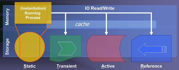
The first category is static data which is comprised of executables, configuration files, models, static images, templates, style sheets, etc. This data usually gets loaded once when a process starts and much of what is needed is instantiated in the systems memory as a running process or cached frequently used templates and images files and therefore IO happens at start up and then less frequently there after. The next category is transient data which is comprised of temporary files, database transaction logs, database redo logs, spools, queues, temporary database tables etc. This data is usually only accessed a few times and then either purged or over-written in a cyclical file. The IO profile is more random and sporadic and in the case of data servers usually works in concert with access to retained active data. The next category is active data which includes RDBMS data, HDMS data, file shares, document or image stores, etc. This is the retained working data set used by an application component and typically involves heavier sequential IO operations. The final category is reference data and includes RDBMS indexes, HDMS directory data and meta data and is generally referenced in concert with access to retained active data to identify what active data needs to be accessed based upon criteria stored in the reference data. Categorizing the file systems/directories specified by a component into one of these categories will help to identify potential data structuring to achieve an isolation of IO to reduce contention and to consolidate similar IO patterns there by increasing sequential IO potential.

Determining a Size Model

Model	Description
Small	50 – 256 GB or up to 1200 IO/s
Medium	256 – 750 GB or up to 1800 IO/s
Large	750 – 5000GB or up to 3600 IO/s
Huge	>5000GB or >3600 IO/s

Now that we know what the application component does and we know what types of data files it uses the next step is to determine how large of an implementation this component is supporting. The size should be made based upon the size of the file spaces and/or the estimated number of IOs. This model should then be used to determine if the file spaces need to be separated and to what extent based upon the storage activity category.

Using OS Storage Abstractions to Optimize Layout and Use

Finally, now that much has been learned about the component being implemented and a determination of file space and implementation size; what mechanism may be used to manage IOs? Most operating systems have facilities for creating logical abstractions of storage. The diagram of OS Storage Abstraction below depicts a typical volume management facility. This is true of HP LVM, AIX Volume Manager and Veritas Volume Manager and is even true of Solaris z-pools and zfs file systems.

These abstraction structures provide the means to limit storage access in three ways. Device groups, Volume Groups or Windows labeled Disks provide a means of isolating IO. The logical partitions are distributed across the presented disks based upon several parameters but all their IO is limited to the devices within the group. The logical partitions and file systems limit data growth and directories provide a logical segregation of files into hierarchies for organizational purposes. Once an implementation size is determined a model may be assigned. In a small model all the storage activity categories may be handled by a single device group. In a medium model the reference and transient data should be placed in a device group and the static and active data placed in another device group. In a large model Static and reference data are placed in one device group, transient data into a second and active data into a third device group and file systems created per specifications. Finally if a component is determined to have a huge IO / Size requirement four or even more device groups should be considered including multiple partitioning of transaction, active and reference data.

Division of the volume groups may be tackled in several ways. One way would be to track all device group names and their purpose and add new device groups based upon the new application components the service or application they are supporting. This becomes more complex in shared service environments where one system may host several instances of a component. An easier way to accomplish this is through using a device group naming convention. With a naming scheme analysts don’t need to know what device groups already exist, at a glance how storage is used on a system can be seen from the device group names and it eliminates the creation of unnecessary volume groups since any new file systems that fall into pre-existing categories will end up being assigned to the appropriate pre-existing device group. Essentially the used device group names are self-tracking since the application of the naming process should result in the same name or a new name when applicable. The implementation of the naming scheme can be automated in a spreadsheet form using lookups based upon the models and categorizations of the file systems requested in the form. The naming scheme I have used has the following form:

• [app abbreviation up to 4 characters][00 Instance number][storage activity category(STAR)][Environment Code]
• example: Oracle People Soft Data Table Production = orps1ap
  Oracle People Soft Index Table Production = orps1rp

Component	Code	Storage Access	Code	Environment	Code
Client	C	Static	S	Development	D
Utility	U	Transient	T	Integration Test	I
Application	A	Active	A	Acceptance Test	A
Data	D	Reference	R	Quality Assurance	Q
				Production	P
				Disaster Recovery	R

Conclusion

Exploring the structures that comprise an application component and then making informed judgments based upon the size of an implementation will result in better performance and a more efficient use of resources. The isolation of IOs by the type of data access will place like data together increasing sequential access potential and decreasing the potential for IO conflicts due to concerted access between active, transient and reference data types.

Bellow is a link to a worksheet which I had created a while ago to determine volume group names based upon data types.

– VG Storage Layout Excel Worksheet